Job preferences

Utku Olcar
is open to work
Job titles
Robotics Engineer · Robotics Software Engineer · Robotics Specialist · Mechatronics Engineer · Embedded Software Engineer
Start date
Immediately, I’m actively applying
Job types
Full-time (I can work remotely)
If you are hiring, leave an email address, please.
“Stewart Platform” 6-DOF Motion Platform Calculations
Details
- Date : November 13, 2019
- Category : Robotic Design and Modelling
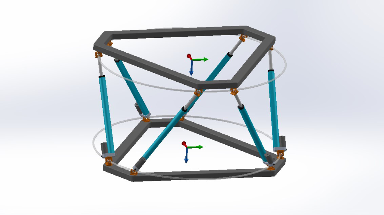
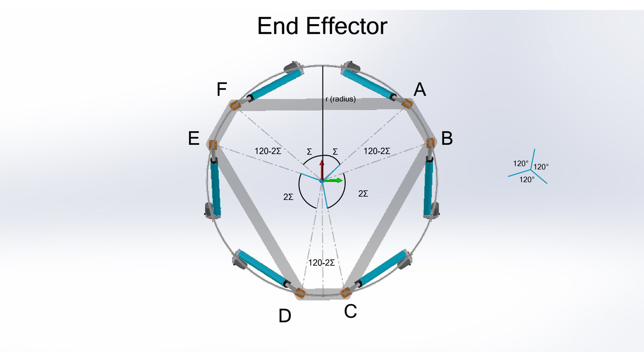
I have a virtually created Stewart Platform that is designed with Solidworks software. I have created to explain how does inverse kinematics works with parallel robots.
The main purpose of the controller's embedded software of this device is that moving the end effector plate to the desired position and the rotation. So, in this study, our inputs will be ;
- The center position of the end effector plate concerning the base plate.
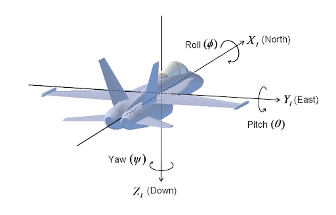
- The Euler Angles (Roll, Pitch, Yaw) of the rotation of the end effector plate, again concerning the base plate's rotation.
If we name the six actuators from A to F, the links are called as
Links = \begin{bmatrix} L { \atop A} \\[1em] L { \atop B} \\[1em] L { \atop C}\\[1em] L { \atop D} \\[1em] L { \atop E} \\[1em] L { \atop F} \\[1em] \end{bmatrix}
Our outputs will be the link lengths of the linear actuators. The length parameters are shown with "Len" ;
Input = \begin{bmatrix} pos X \\[1em] pos Y \\[1em] pos Z \\[1em] \phi \\[1em] \theta \\[1em] \psi \\[1em] \end{bmatrix}
Output = \begin{bmatrix} Len { \atop A} \\[1em] Len { \atop B} \\[1em] Len { \atop C} \\[1em] Len { \atop D} \\[1em] Len { \atop E} \\[1em] Len { \atop F} \\[1em] \end{bmatrix}
The base plate's frame will be frame 0 and the end effector plate frame will be frame 1.
The joint points of the links are named for base joints :
Base Joints = \begin{bmatrix} A{ \atop 0} \\[1em] B { \atop 0} \\[1em] C { \atop 0} \\[1em] D { \atop 0} \\[1em] E { \atop 0} \\[1em] F { \atop 0} \\[1em] \end{bmatrix}
End Effector Joints = \begin{bmatrix} A{ \atop 1} \\[1em] B { \atop 1} \\[1em] C { \atop 1} \\[1em] D { \atop 1} \\[1em] E { \atop 1} \\[1em] F { \atop 1} \\[1em] \end{bmatrix}
Let's begin to solve the problem. To find the link lengths, we need the 3-dimensional position differences of two joint of the links. To find them, we need all calculated positions concerning the base frame.
Output = Link Lengths =
\begin{bmatrix}
Len { \atop A} =\begin{vmatrix} A{0 \atop 1} - A{0 \atop 0} \end{vmatrix} \\[1em]
Len { \atop B} =\begin{vmatrix} B{0 \atop 1} - B{0 \atop 0} \end{vmatrix} \\[1em]
Len { \atop C} =\begin{vmatrix} C{0 \atop 1} - C{0 \atop 0} \end{vmatrix} \\[1em]
Len { \atop D} =\begin{vmatrix} D{0 \atop 1} - D{0 \atop 0} \end{vmatrix} \\[1em]
Len { \atop E} =\begin{vmatrix} E{0 \atop 1} - E{0 \atop 0} \end{vmatrix} \\[1em]
Len { \atop F} =\begin{vmatrix} F{0 \atop 1} - F{0 \atop 0} \end{vmatrix} \\[1em]
\end{bmatrix}
We know the positions of points concerning their own frame (base point concerning base frame, end effector points concerning end effector frame). All we need is the 3D positions of the end effector joints concerning the base frame.
The positions of the end effector joints with respect to the end effector frame are constant.
A{1 \atop 1} =
\begin{pmatrix}
x{ \atop a1} ,& y{ \atop a1} ,& z{ \atop a1}
\end{pmatrix}
The positions of base joints with respect to the base frame are constant too.
A{0 \atop 0} =
\begin{pmatrix}
x{ \atop a0} ,& y{ \atop a0} ,& z{ \atop a0}
\end{pmatrix}
We need the transformation of these two frames from 0 to 1. To describe the transformation matrix, we need the rotation matrix and the position of the end effector frame with respect to the base.
T{0 \atop 1} =
\begin{bmatrix}
R{0 \atop 1} & P{0 \atop 1} \\[1em]
(0,0,0) & 1 \\[1em]
\end{bmatrix}
The position is given as input. We put that input directly to the right column.
P{0 \atop 1} = \begin{bmatrix} pos X \\[1em] pos Y \\[1em] pos Z \\[1em] . \end{bmatrix}
The rotation matrix will be generated;
R{0 \atop 1} = R{ \atop z}(\psi) R{ \atop y}(\theta) R{ \atop x}(\phi) = \begin{bmatrix} \cos \psi & -\sin \psi & 0 \\[1em] \sin \psi & \cos \psi & 0 \\[1em] 0 & 0 & 1 \\[1em] \end{bmatrix} \begin{bmatrix} \cos \theta & 0 & \sin \theta \\[1em] 0 & 1 & 0 \\[1em] -\sin \theta & 0 & \cos \theta \\[1em] \end{bmatrix} \begin{bmatrix} \cos \phi & -\sin \phi & 0 \\[1em] \sin \phi & \cos \phi & 0 \\[1em] 0 & 0 & 1 \\[1em] \end{bmatrix} \\[1em]
If we multiply all matrix, the result would be ;
R{0 \atop 1} = \begin{bmatrix} \cos \psi \cos \theta & \cos \psi \sin \theta \sin \phi - \sin \psi \cos \phi & \cos \psi \sin \theta \cos \phi + \sin \psi \sin \phi \\[1em] \sin \psi \cos \theta & \sin \psi \sin \theta \sin \phi +\cos \psi \cos \phi & \sin \psi \sin \theta \cos \phi - \cos \psi \sin \phi \\[1em] - \sin \theta & \cos \theta \sin \phi & \cos \theta \cos \phi \\[1em] \end{bmatrix} \\[1em]
So the Transformation Matrix has been described :
T{0 \atop 1} = \begin{bmatrix} \cos \psi \cos \theta & \cos \psi \sin \theta \sin \phi - \sin \psi \cos \phi & \cos \psi \sin \theta \cos \phi + \sin \psi \sin \phi & pos X \\[1em] \sin \psi \cos \theta & \sin \psi \sin \theta \sin \phi +\cos \psi \cos \phi & \sin \psi \sin \theta \cos \phi - \cos \psi \sin \phi & pos Y \\[1em] - \sin \theta & \cos \theta \sin \phi & \cos \theta \cos \phi & pos Z \\[1em] 0 & 0 & 0 & 1 \\[1em] \end{bmatrix} \\[1em]
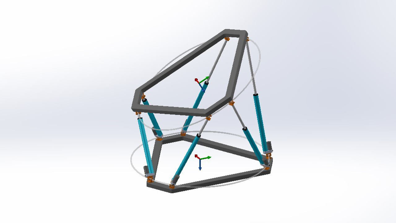
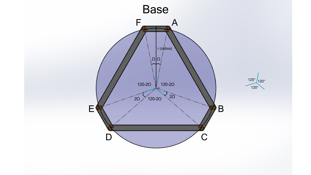
Okey. Let's calculate the positions for link joints. The calculations before this step were the same for all the parallel robot systems. Starting with this step, we will calculate the Stewart Platform's geometry. Every Stewart Platform has some similarities about the geometry. So we will calculate the positions with these common assumptions.
pos A { \atop 0} = ( X{ \atop A0}, Y{ \atop A0}, 0 )
pos B { \atop 0} = ( X{ \atop B0}, Y{ \atop B0}, 0 )
pos C { \atop 0} = ( X{ \atop C0}, Y{ \atop C0}, 0 )
pos D { \atop 0} = ( X{ \atop D0}, Y{ \atop D0}, 0 )
pos E { \atop 0} = ( X{ \atop E0}, Y{ \atop E0}, 0 )
pos F { \atop 0} = ( X{ \atop F0}, Y{ \atop F0}, 0 )
Fill the X, Y data with the "r" and "Ω" variables ;
pos A {0 \atop 0} = ( r \sin \Omega, r \cos\Omega, 0 )
pos B{0 \atop 0} = ( r \sin (120-\Omega),r \cos(120-\Omega) , 0 )
pos C {0 \atop 0} = (r \sin (120+\Omega), r \cos(120+\Omega), 0 )
pos D{0 \atop 0} = ( r \sin (240-\Omega), r \cos (240-\Omega), 0 )
pos E{0 \atop 0} = ( r \sin (240+\Omega), r \cos(240+\Omega), 0 )
pos F{0 \atop 0} = ( r \sin (360-\Omega), r \cos(360-\Omega), 0 )
End Effector :
posA{1 \atop 1} = ( r \sin \Sigma, r \cos\Sigma, 0 )
pos B{1 \atop 1}= ( r \sin (120-\Sigma),r \cos(120-\Sigma) , 0 )
pos C{1 \atop 1} = (r \sin (120+\Sigma), r \cos(120+\Sigma), 0 )
pos D {1 \atop 1} = ( r \sin (240-\Sigma), r \cos (240-\Sigma), 0 )
pos E{1 \atop 1} = ( r \sin (240+\Sigma), r \cos(240+\Sigma), 0 )
pos F{1 \atop 1} = ( r \sin (360-\Sigma), r \cos(360-\Sigma), 0 )
These positions are calculated with respect to the end effector frame. We need these positions with respect to the base frame.
P{0 \atop1} = T {0 \atop 1} P{1 \atop 1}
So we can calculate these using the Transformation Matrix easily using this formula.
For example :
pos A{0 \atop 1} = \begin{bmatrix} \cos \psi \cos \theta & \cos \psi \sin \theta \sin \phi - \sin \psi \cos \phi & \cos \psi \sin \theta \cos \phi + \sin \psi \sin \phi & pos X \\[1em] \sin \psi \cos \theta & \sin \psi \sin \theta \sin \phi +\cos \psi \cos \phi & \sin \psi \sin \theta \cos \phi - \cos \psi \sin \phi & pos Y \\[1em] - \sin \theta & \cos \theta \sin \phi & \cos \theta \cos \phi & pos Z \\[1em] 0 & 0 & 0 & 1 \\[1em] \end{bmatrix} \begin{bmatrix} r \sin \Sigma \\[1em] r \cos\Sigma \\[1em] 0 \\[1em] 1 \\[1em] \end{bmatrix}
Len A = magnitude of ( pos A{0 \atop 1} - pos A{0 \atop 0} )
Len B = magnitude of ( pos B{0 \atop 1} - pos B{0 \atop 0} )
Len C = magnitude of ( pos C{0 \atop 1} - pos C{0 \atop 0} )
Len D = magnitude of ( pos D {0\atop 1} -pos D {0 \atop 0} )
Len E = magnitude of ( pos E {0 \atop 1} - pos E{0 \atop 0} )
Len F = magnitude of ( pos F {0 \atop 1} - pos F{0 \atop 0} )
Reference:
- Mark ,S, Seth, H. and M., Vidyasagar, 2005. Robot Modeling and Control. 1th ed. Wiley
Related Posts
Check out my all posts-
December 1, 2019
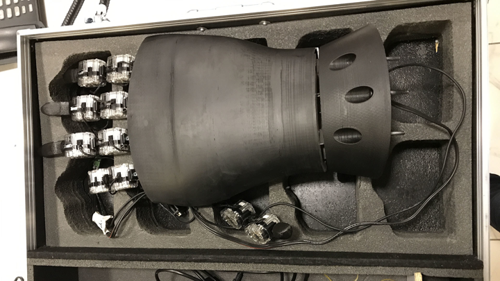
How to Make A Teleoperated Robotic Hand? This is an approximately 50 cm lenght robotic hand, designed and produced ...
Category ROBOTIC DESIGN AND MODELLING
-
Februray 2, 2017
The main idea is that adding external forces to the joint points of the robotic arm. If any obstacle (object) is close e...
Category ROBOTIC CALCULATIONS
-
November 3, 2017
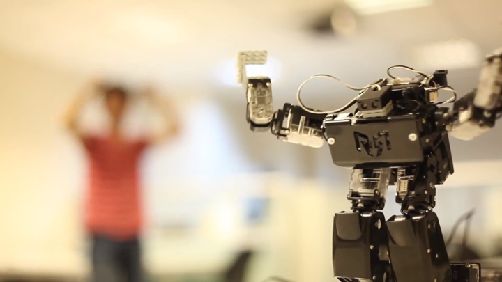
Teleoperation systems which imitate human movements and controlled by a human body are infrequent projects and these wor...
Category ROBOTIC CALCULATIONS
Comments
RashR
3/20/2025
"posA0 =(X A0,Y A0,0) posA 00=(rsinΩ,rcosΩ,0)" can you tell me how i can get values for x, y, Ω, posX, posY, and posZ. can you explain it using example.
sumedh
10/31/2023
the answer we are gonna get will still be a 4x1 matrix right, where is the length of the actuator here?
sumedh
10/31/2023
the answer we are gonna get will still be a 4x1 matrix right, where is the length of the actuator here?
11/13/2019
utku olcar
6-DOF Robot, Inverse Kinematics, Kinematics, Parallel Robots, Robotics, Rotation Matrix, Stewart Platform, Transform Matrix Robotic Calculations, Robotic Design and Modelling
3 Comments